Planning through
regimes.
Regime models promise to hold less risk when markets turn turbulent. I tested them the way an allocator would have lived them: every parameter and state estimate dated by what was knowable, US data back to 1926, and trading costs anchored to a century of measured costs. Then I worked out why regime signals fail in execution, and what fixes it.
Most of the published edge is information nobody had
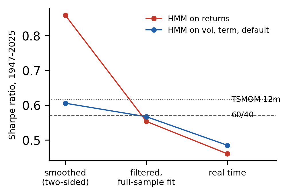
Hold one model fixed and shrink only what it knows. A two-state hidden Markov model on stock and bond returns earns a Sharpe ratio of 0.86 when each month uses the smoothed regime probability that regime papers usually plot. With full-sample parameters but probabilities filtered in time it earns 0.55. Fit in real time it earns 0.46, below a plain 60/40 portfolio (0.57). Across 35 real-time configurations (four feature sets and returns, two to four regimes, three execution rules), none beats 60/40; simple trend rules do (0.62 to 0.64).
The state of the art, outside its sample
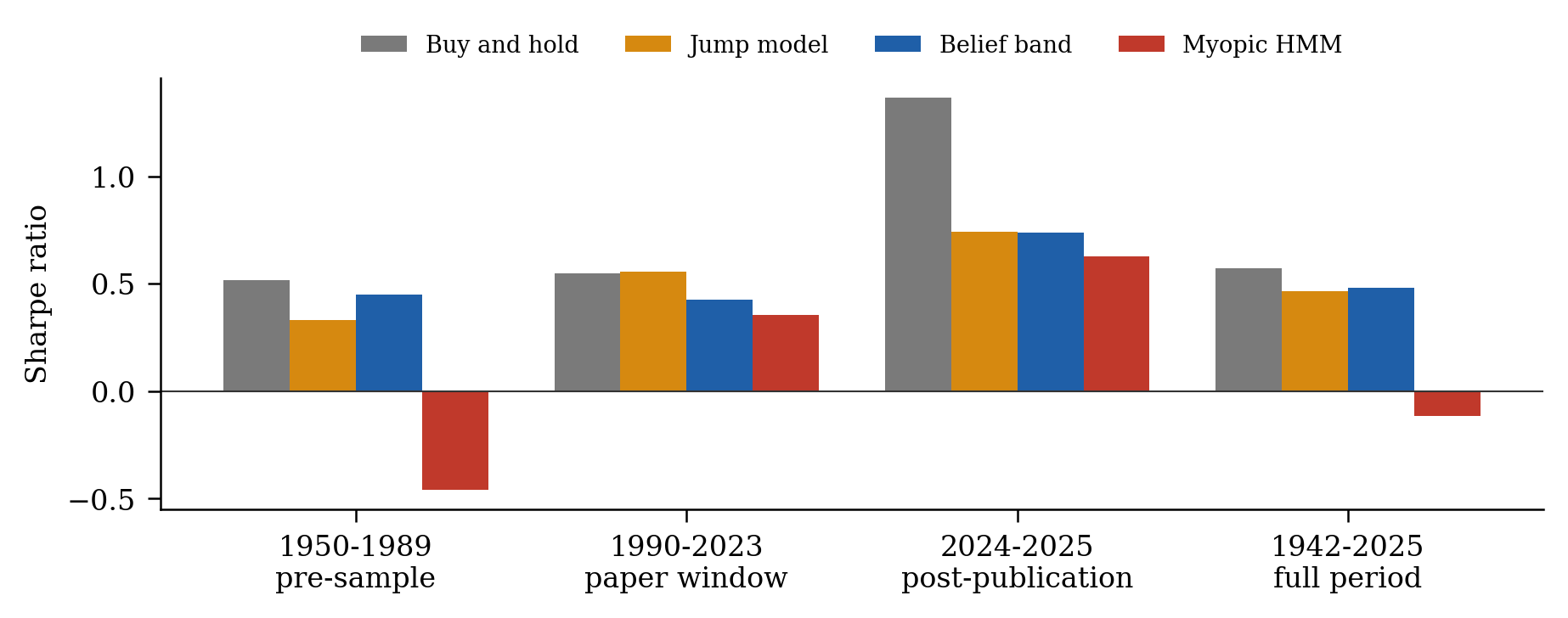
Statistical jump models are the current best published method, reporting a Sharpe ratio of 0.68 against 0.48 for the S&P 500 over 1990-2023. I re-implemented the protocol from the paper and the authors' code (features, clipping, penalty grid, eight-year validation, one-day delay). On its own window it reproduces the drawdown cut (-30% against -55%) and a smaller Sharpe gain (0.51 against 0.49). On 1950-1989, which the method never saw, it earns 0.35 against buy-and-hold's 0.59. In four other developed markets since 2009 its Sharpe ratio is at or below 0.10 in seven of eight cases.
Why regime signals die in execution: a cube-root law
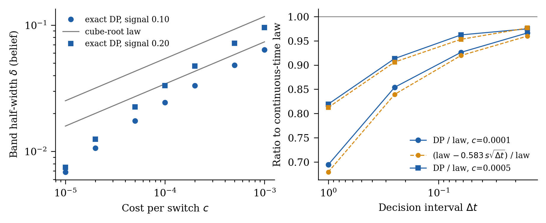
Treat the regime as hidden and the investor's belief as the state. Without trading costs, the belief problem has a trivial answer: act myopically on today's belief, because nothing you do changes what you will learn. That is why the planner in my original course project collapsed to a simple rule. Add the current holding to the state and a proportional cost to every switch, and the answer changes: hold your position inside a band of beliefs, and trade only at its edges. Value matching and smooth pasting give the band's half-width:
Here K is the cost of a switch, s the speed at which the belief moves, and g how fast the payoff of being invested falls as turbulence becomes more likely. The 0.5826 is −ζ(½)/√(2π), the same constant that corrects discretely monitored barrier options. Exact dynamic programming confirms the law to within 2%, and on 186 refits of the real daily model the corrected law predicts the bands the solver chose (median ratio 0.97).
Planned, the same signal survives its own trading
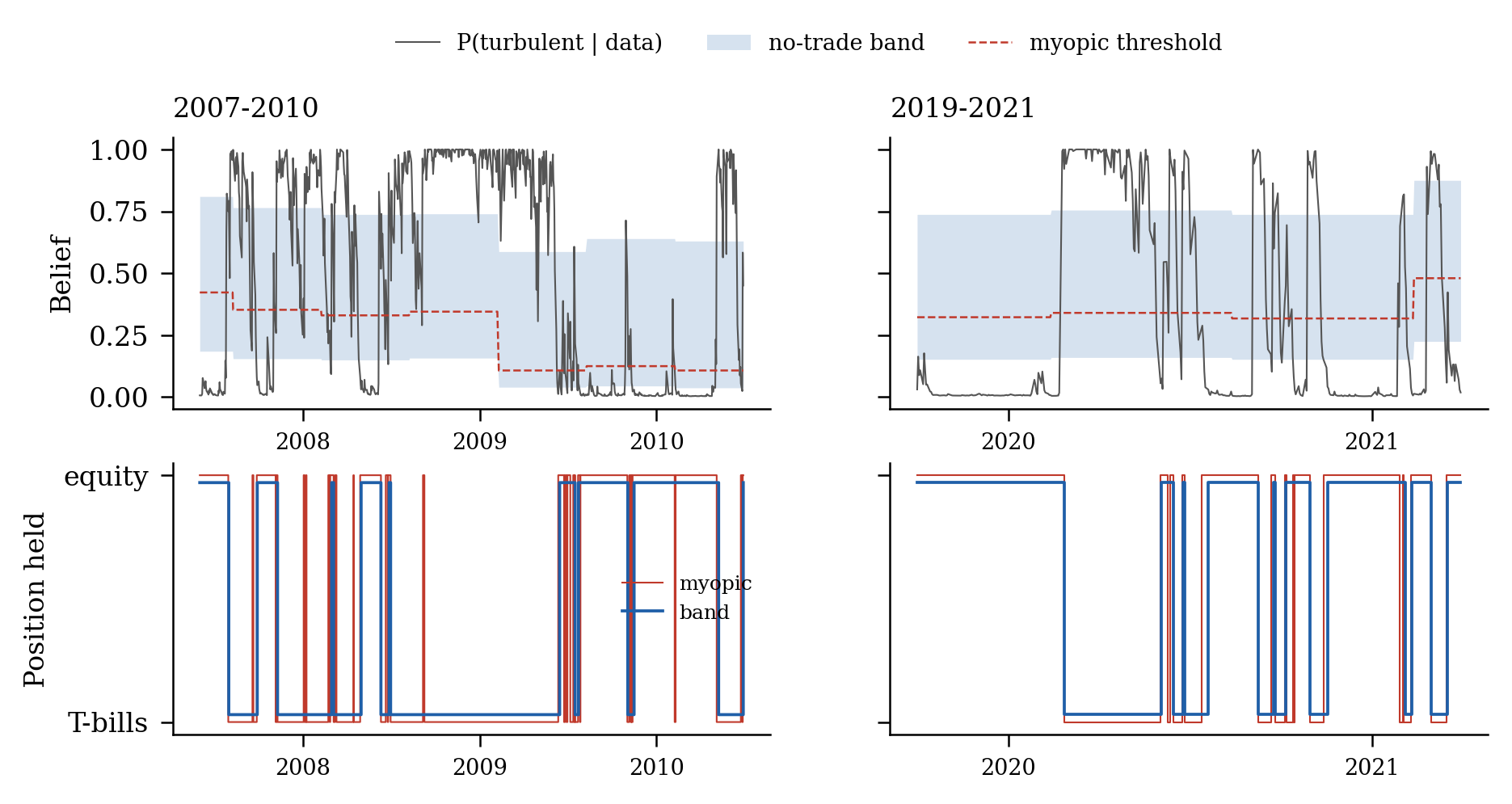
Acting myopically on a daily regime belief means 13 switches a year. At historical costs that loses 94% from peak. The band policy, solved exactly from the fitted model with nothing tuned on outcomes, trades three to eight times a year and keeps a Sharpe ratio between 0.48 and 0.55 at every cost level. It ties the jump model statistically and roughly halves buy-and-hold's drawdown. It does not beat the market: in real time, regimes are a risk-management tool, and only a planned one is worth running.
What it means for an allocator
The band is set by the cost of the instrument you act with. For index futures and ETFs it nearly vanishes and myopic switching is close to optimal. For institutional equity and corporate bonds it covers much of the belief range. At the discounts at which private-equity fund stakes trade in the secondary market (8% for buyout in 2025, 46% on average in 2009) the optimal policy never sells, whatever the belief. That is the denominator effect explained: tolerating an overweight, or raising the target, is the band at work.
| Instrument | One-way cost | Hold equity while P(turbulent) is in | Switches / yr |
|---|---|---|---|
| E-mini S&P 500 futures | 0.2 bp | about 0.50 (myopic) | 10.8 |
| 10-year Treasury | 0.9 bp | 0.46 to 0.57 | 9.5 |
| Large-cap equity, institutional | 8.9 bp | 0.32 to 0.76 | 5.9 |
| Investment-grade corporates | 38 bp | 0.17 to 0.89 | 4.1 |
| US equity, 1953-1975 | 100 bp | 0.08 to 0.96 | 3.0 |
| Buyout fund stake, secondary 2025 | 8% | never sells | 0 |
| Any PE stake, secondary 2009 | 46% | never sells | 0 |
Limits
- The daily study uses one regime model family on equities against T-bills; multi-asset daily belief spaces are left for later.
- The historical cost schedule interpolates between documented anchors and assumes bond costs at half of equity costs.
- The law is leading-order in the cost; daily beliefs jump, which is why the discrete correction matters.
- Nothing here is investment advice.